In the early 1970s Brenner, Deen, and others performed a series of foundational experiments on Munich-Wistar rats. These rats were chosen because they had glomeruli on their cortical surface which allowed researchers to measure tubular and capillary flow, pressure, and composition directly via micropuncture. 50 years later, the mathematical model created by the authors remains accurate, relevant, and forms the basis of our understanding of glomerular filtration.
The model conceptualizes the glomerular capillary bed as a dimensionless semiporous cylinder traversing through Bowman’s space. The hydrostatic pressure (PGC) in this idealized glomerular capillary is considered to remain near-constant throughout its length. The pressure in Bowman space (PBS) is also considered to remain relatively constant. What varies over the length of the glomerular capillary, in a nonlinear manner, is the oncotic pressure (πGC). The oncotic pressure in Bowman’s space (πBS) is presumed to be zero (Figure 1).
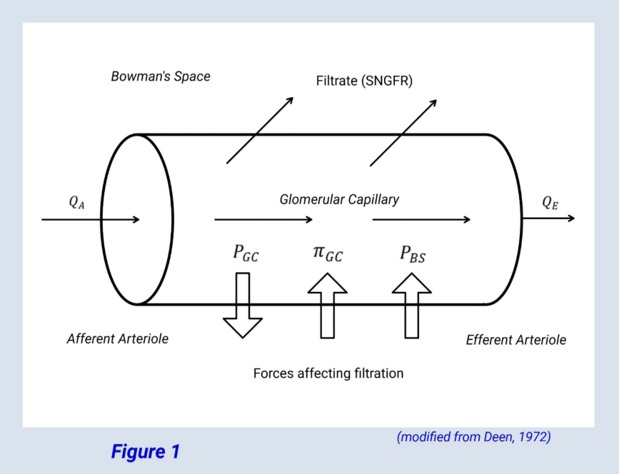
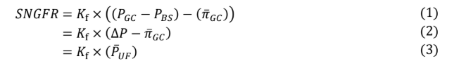
Another variable in the model Is the filtration constant (KKf), which is the product of the glomerular capillary filtration coefficient and surface area. The filtration constant, combined with the three pressures described above give the following equations for SNGFR.
Again, it is the glomerular capillary oncotic pressure, which varies in a nonlinear way along the glomerular capillary, which is somewhat more complicated to quantify. This in turn makes mean ultrafiltration pressure more difficult to quantify.
Figure 2 depicts ultrafiltration pressure (represented by the area outlined in light violet) along the glomerular capillary in the Munich-Wistar rat in three different volume states, hypovolemia, euvolemia, and hypervolemia. In each volume state, the mean ultrafiltration pressure corresponds with the area outlined in light violet.
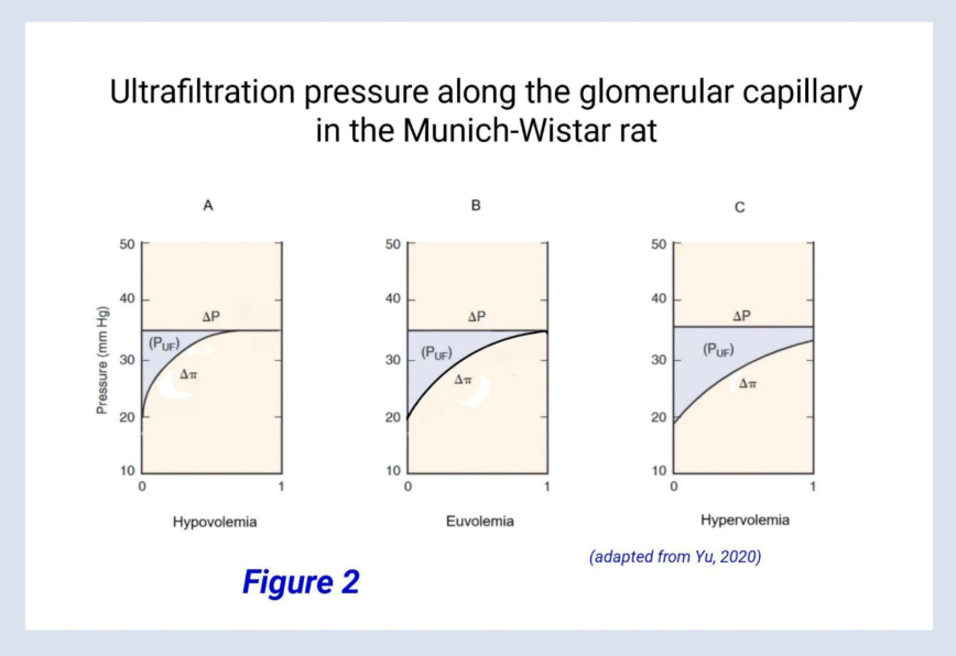
Note that in Figures 2A and B, oncotic (inward) pressure equals hydrostatic (outward) pressure by the end of the idealized glomerular capillary, and these pressures become equal well before the end of the capillary in hypovolemia. When these pressures become equal, a state defined as filtration equilibrium, net filtration ceases. Filtration equilibrium is reached under normal physiologic conditions in rats and several other small mammals but is not reached in larger mammals such as dogs or humans. This will be revisited later, but for now, suffice it to say that reaching filtration equilibrium simplifies the math in the Munich-Wistar rat model.
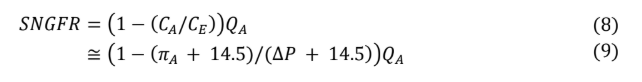
Since no protein is filtered through the idealized glomerular capillary, and in accordance with the law of mass conservation, the amount of protein then enters the glomerular capillary must equal the amount that leaves. Since there will be a filtrate loss over the course of the glomerular capillary, the protein concentration at the efferent arteriole (CE) will be higher than at the afferent arteriole (CA), as glomerular capillary flow will be lower by an amount equal to SNGFR.
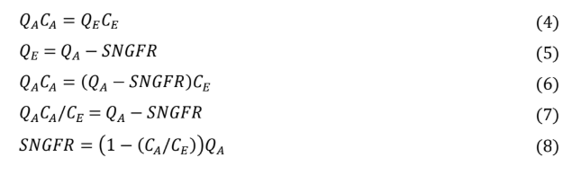
Substituting equation 5 Into equation 4 yields equation 6, which can then be simplified to equation 8. In all instances, whether filtration equilibrium is reached or not, equation 8 remains accurate. However, in the absence of filtration equilibrium, modeling protein concentration along the glomerular capillary and calculating (CE) requires advanced mathematics beyond the scope of this review.
Because filtration equilibrium is achieved in the Munich-Wistar rat, the model may be pursued further, as the math is more manageable. Referring to equation 3, recall that SNGFR equals the product of the filtration constant and mean ultrafiltration pressure, or SNGFR = Kf × (PUF). Referring to figure 2, recall that mean ultrafiltration pressure (PUF) is proportional to the areas outlined in light violet. Also recall that filtration equilibrium Is achieved in the hypovolemic and euvolemic states (A, B).
According to the Brenner-Deen model, three values are required to define mean ultrafiltration pressure. These are afferent arteriolar flow (QA) and oncotic pressure (πA), and hydrostatic pressure (∆P). This is also evident from figure 2 as oncotic and hydrostatic pressures form two borders of the light violet triangles. And in going from A to C, the light violet areas increase due to progressively increasing flow.
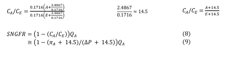
Recalling equation 8, SNGFR can be defined in terms of the ratio of protein concentrations between the afferent and efferent arterioles. Given the condition of filtration equilibrium, hydrostatic pressure must equal oncotic pressure by the end of the glomerular capillary (∆P = πE ). However, the relationship between protein concentration to oncotic pressure Is a nonlinear one, leading again to some relatively complicated math. Fortunately, over the range of utility for the model, linear regression approximation remains fairly accurate (see appendix).
Based on equation 8, using this linear regression approximation yields the following.
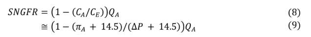
Equation 9 has three of the four values required to calculate SNGFR. Because filtration equilibrium is assumed to be reached, the filtration constant (Kf) does not appear in the equation. From any point of filtration equilibrium, an increase in the filtration constant results in a proportional decrease in mean filtration pressure (light violet triangle gets smaller) so that SNGFR does not change. Likewise, any decrease in the filtration constant results in a proportional increase in mean filtration pressure (light violet triangle gets larger), so that again SNGFR does not change, up to the point that the filtration constant is low enough that filtration equilibrium no longer occurs, at which time the above equation is no longer applicable.
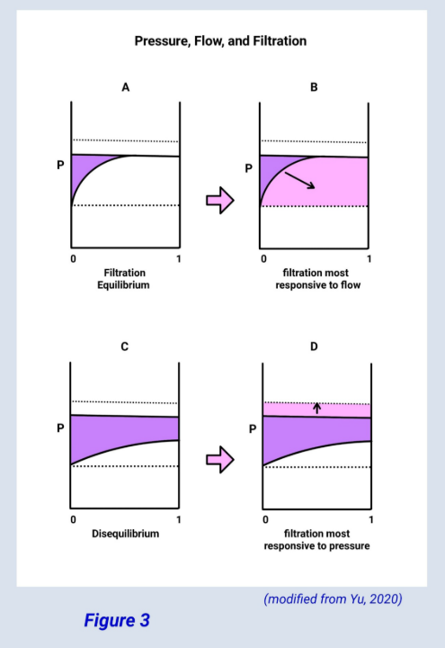
Figure 3 (below) graphically shows that when filtration equilibrium is being reached filtration is most influenced by glomerular flow, as opposed to disequilibrium, where filtration is more responsive to pressure.
Current textbooks still use the data, model, and figures of Brenner and Deen to explain single nephron GFR some 50 years after their work was first published. This is testament to the timeless genius of their work.
Appendix
What follows is the mathematical derivation of equation 9 from equation 8.
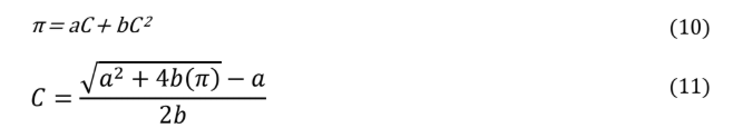
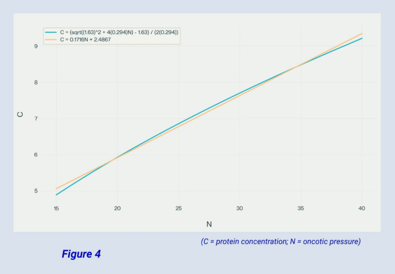
Equation 10 is a quadratic adaptation of the Landis-Pappenheimer equation used to relate protein concentration (C) to plasma oncotic pressure (π). Solving for C in terms of π yields equation 11.
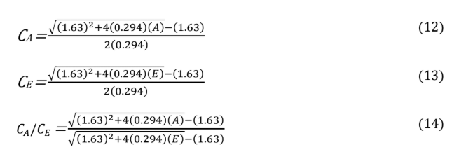
Using (1.63) for a and (0.294) for b and stipulating that πA = A and πE = E yields equations 12 and 13. Dividing these two equations yields an accurate expression for CCAA/CCEE which unfortunately is quite cumbersome mathematically.
At this point, a linear approximation for (C) In terms of (π) helps to make the math more manageable (see Figure 4 below). Using the linear approximation, equations 13 and 14 become equations 15 and 16. And equation 14 becomes equation 17 and ultimately equation 18.
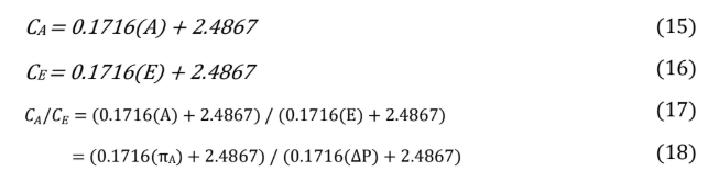
From here, some algebraic manipulation yields equation 9.
References
- Deen W et al. (1972) A model of glomerular ultrafiltration in the rat American Journal of Physiology 223(5) p.1178-83.
- Yu ASL et al. (2020) Brenner and Rector’s The Kidney, Eleventh Ed.
- Oken DE (1982) An analysis of glomerular dynamics in rat, dog, and man KI 22(2) p.136-45.
- Brenner B et al. (1976) Determinants of glomerular filtration rate. Ann Rev Physiol 38(1) p.9-19.
- Pollak MR et al. (2014) The glomerulus, the sphere of influence CJASN 9(8) p.1461-69.